Info theory for comp neuro | Annie G. Bryant

Illustrative tutorial to accompany our preprint

🔗 GitHub Repository: https://github.com/anniegbryant/info_theory_visuals

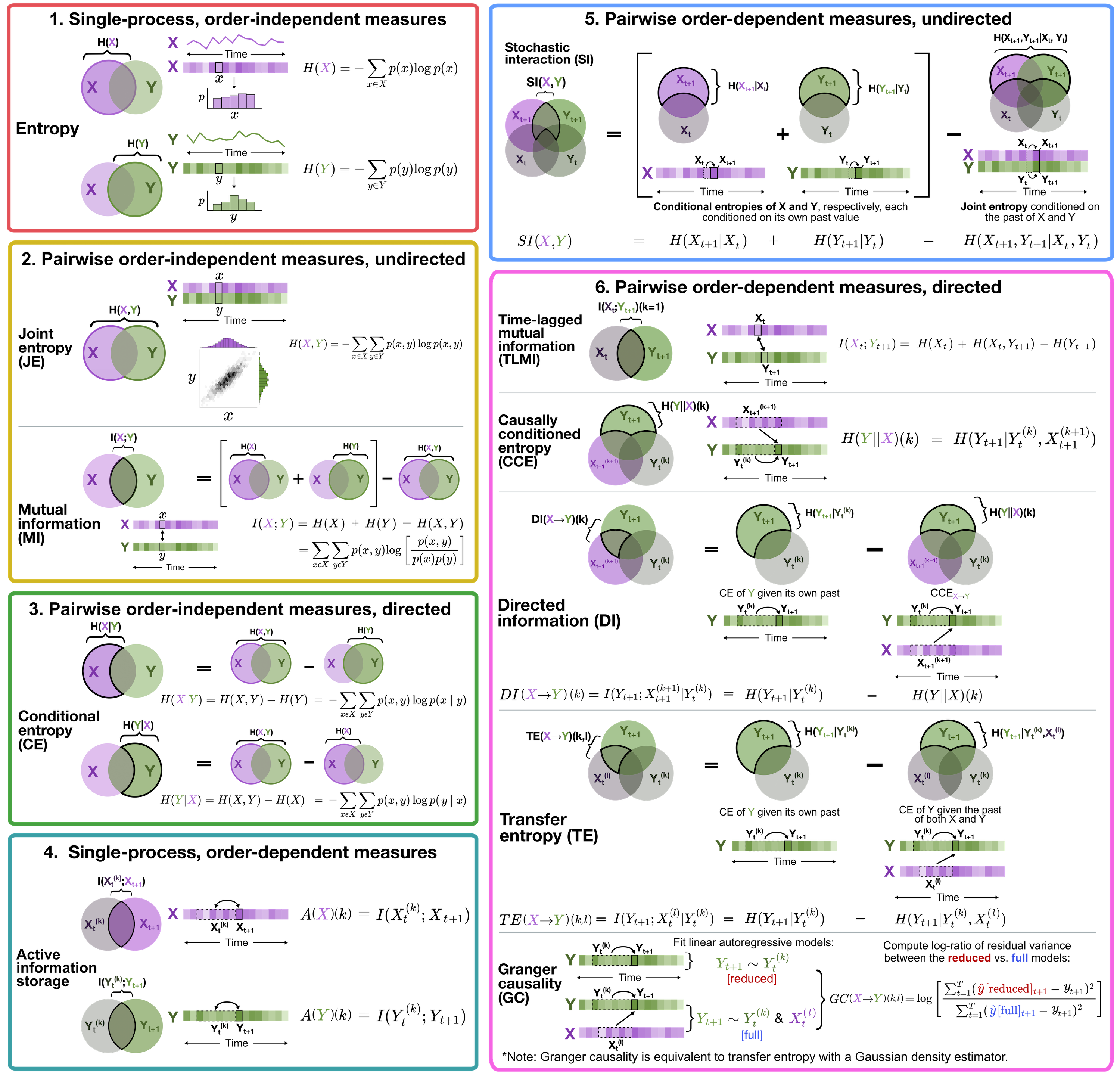
This repository is designed as a simple guide to computing information-theoretic time-series measures covered in our (preprinted) review, ‘Unifying concepts in information-theoretic time-series analysis’.

We work through the computation and interpretation of 11 measures (2 single-process and 9 pairwise) using two open-source software packages:

Java Information Dynamics Toolkit (JIDT); and
Python toolkit of statistics for pairwise interactions (pyspi)

Both are implemented in python, either directly (pyspi) or with a wrapper interface to java using jpype (JIDT).

About the dataset in this guide

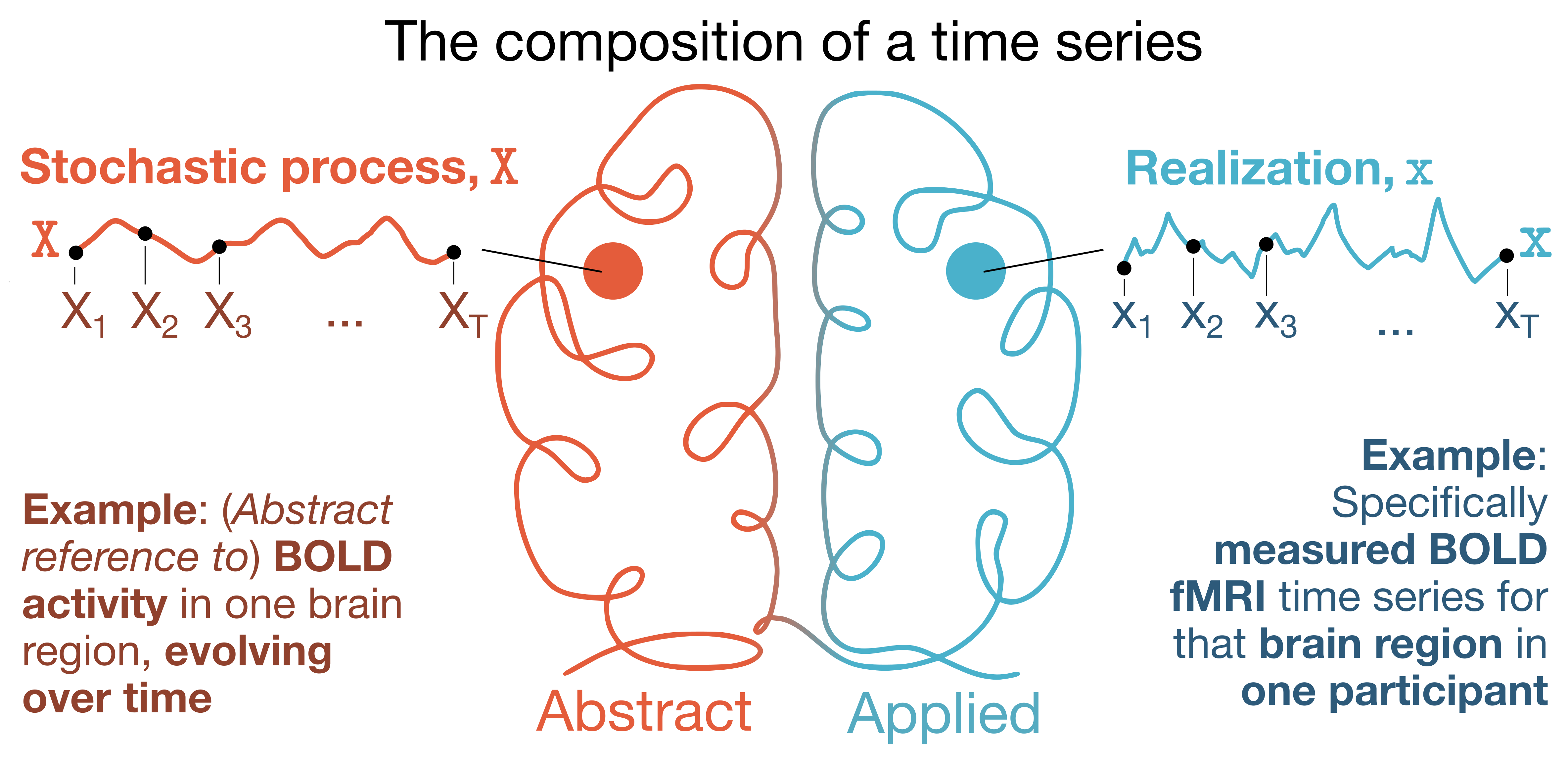
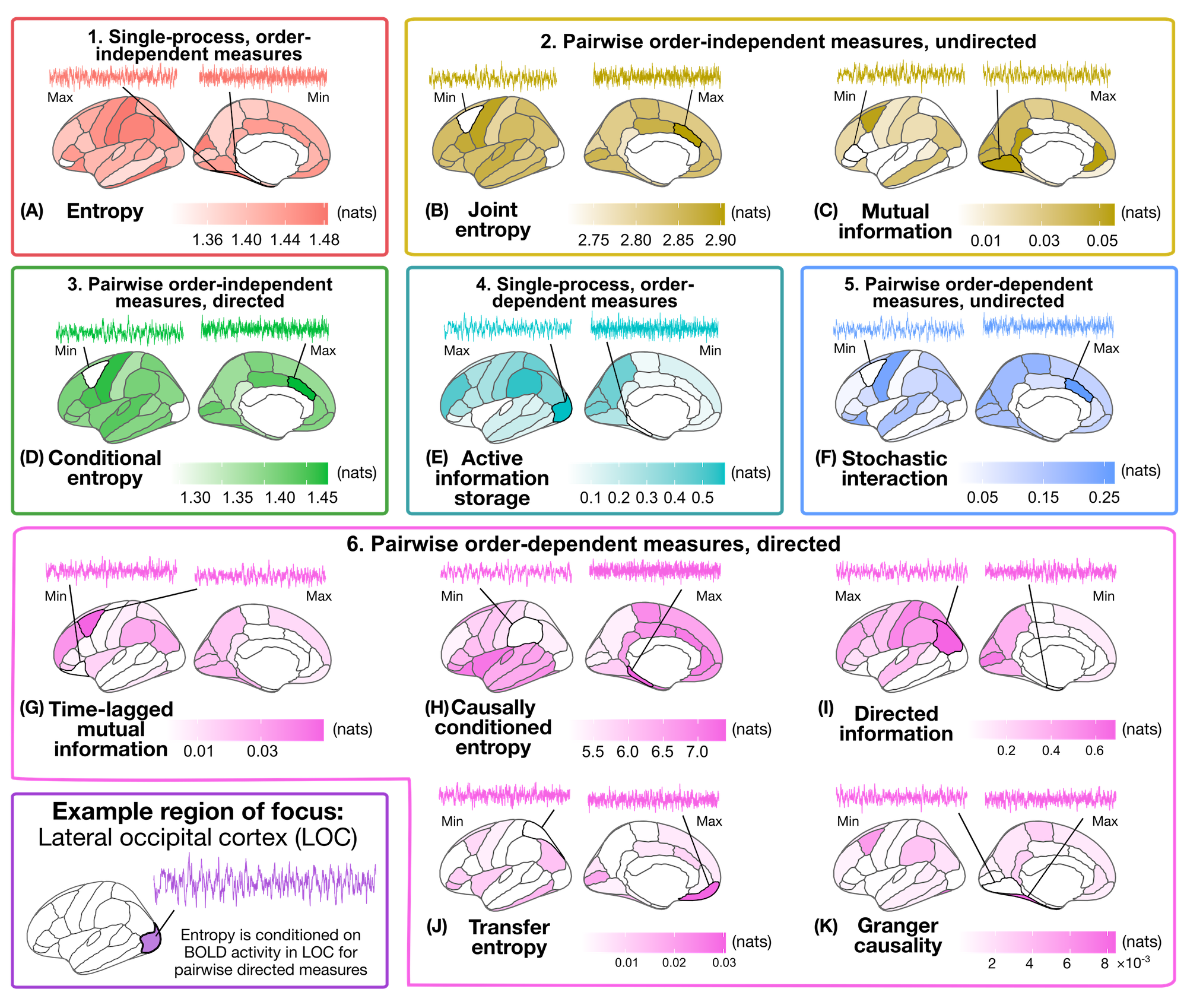
For our illustrative case study, we’re working with resting-state BOLD fMRI data from one participant in the Human Connectome Project S1200 release (ID ‘298051’, selected at random). This resting-state fMRI dataset was preprocessed in ‘Timescales of spontaneous fMRI fluctuations relate to structural connectivity in the brain’ by John Fallon et al. Network Neuroscience (2020), where details about imaging acquisition, preprocessing, and data availability are all described. Here, we’ve used the 68-region Desikan-Killiany cortical parcellation atlas, focusing on just one hemisphere (left) for simplicity. The resting-state fMRI time series data for this participant (68 regions $\times$ 1200 timepoints) is included in this repository under data/HCP_298051_rsfMRI_DesikanKilliany_TS.csv.

This pipeline is modality-agnostic, meaning you can adapt this code to datasets of different spatial and/or temporal measurement scales, too.

📚Prereqs to run this code

Not too much homework needed to get up and running here, fortunately! While JIDT is standalone software, it is also bundled as part of pyspi, so you will have both packages once you get pyspi on your computer.

You can install pyspi directly with pip; however, we recommend that you clone the GitHub repository to your local machine and then install from your cloned version, just so that you know precisely where your JIDT library is 😊

To clone pyspi, simply run:

git clone https://github.com/DynamicsAndNeuralSystems/pyspi.git

You can then install the python package by running:

# navigate to the freshly cloned repo
cd pyspi 
pip install .

While you’re in there, navigate to the folder pyspi/lib/jidt and make sure you see the file infodynamics.jar. That’s the executable Java file for JIDT, which we’ll call from python using jpype.

That’s pretty much it! To test that pyspi installed correctly, a simple sanity check might look like (in Python):

from pyspi.calculator import Calculator

# Instantiating a Calculator object will load all of the measures computed by default in pyspi
# Meaning, if there is any issue it should be flagged with this
calc = Calculator()

Data visualization prerequisites

If you would like to generate the same type of cortical surface visuals in our preprint:

You’ll need to have a working installation of R and the packages tidyverse, ggseg, cowplot, and patchwork packages. They can be installed within R from the terminal (including the one within RStudio) using:

install.packages(c('tidyverse', 'ggseg', 'cowplot', 'patchwork'))

If you want to interactively run the data visualization code in this repository, please note that we’ve included both python and R code in one Jupyter notebook. This is super useful for data wrangling between the two languages, though in its current form, this also means you will need to install the rpy2 package in python:

pip install rpy2

Sometimes this can be a bit of a headache depending on your operating system; worst case, you can copy–paste code into Python/R separately from the Jupyter notebook (described below) if you can’t get rpy2 installed on your computer.

🏃‍♀️Running the code

Once you’ve got pyspi installed and got eyes on the infodynamics.jar file, you’re all set to start computing your information-theoretic time-series measures! There are two steps to this:

Computing the measures

All code to compute the 11 information-theoretic time-series measures from the example resting-state fMRI dataset is provided in fMRI_compute_infotheory_measures.py. You can take a look at the pre-computed measures in data/HCP_298051_rsfMRI_infotheory_measures.csv for a sense of what the results should look like. If you want to compute the measures yourself for the same dataset, just delete (or relocate) the pre-computed measures and run the python script as:

python3 fMRI_compute_infotheory_measures.py

Visualizing the measures on the left hemisphere cortical surface

Whether you’ve computed the information-theoretic time-series measures yourself or would rather stick with the pre-computed results we provided, the final step is to visualize the resulting measures in the brain!

Check out the Jupyter notebook fMRI_analyze_infotheory_measures.ipynb, which loads in the information-theory measure results for this example participant and visualizes them on the left cortical surface using the ggseg package.

Note that this guide is admittedly cortico-centric, such that the visualization code will need to be tweaked a bit for non-cortical structures. (n.b., if you’re in the market for a similar style subcortex parcellation viz tool, I put together a simple Python package for this that you might like 😇)